
Introduction
This PySpark notebook introduces Spark GraphFrames.
The dataset
SNAP: https://snap.stanford.edu/data/egonets-Facebook.html
Dataset description:
- Nodes 4039
- Edges 88234
Abstract from Stanford’s website: This dataset consists of ‘circles’ (or ‘friends lists’) from Facebook. Facebook data was collected from survey participants using a Facebook app. The dataset includes node features (profiles), circles, and ego networks.
Facebook data has been anonymized by replacing the Facebook-internal ids for each user with a new value. Also, while feature vectors from this dataset have been provided, the interpretation of those features has been obscured. For instance, where the original dataset may have contained a feature “political=Democratic Party”, the new data would simply contain “political=anonymized feature 1”. Thus, using the anonymized data it is possible to determine whether two users have the same political affiliations, but not what their individual political affiliations represent.
For this article, the data files has been downloaded, cleaned from duplicate data and properly formatted in csv format for better handling. You can download the vertices file from here and the edges from here.
All files, including this article as a Python notebook and draft D3js html code can be downloaded from here. Thanks!
Let’s start our introduction to GraphFrames. The following assumes that you have a PySpark interactive console available.
RDD (Resilient Distributed Datasets)
- It is the building block of spark. All data abstractions, such as DataFrames and GraphFrames, are interprested (transformed) in RDDs.
- RDD is lazily evaluated immutable parallel collection of objects normally exposed with lambda functions.
- RDDs are simple to use and expose an Object Oriented like API. See Spark Programming Guide.
- Its main disadvantage is performance limitations. Being in-memory JVM objects, RDDs involve overhead of Garbage Collection and Java Serialisation which become expensive when data grows.
Loading our edges and vertices looks like:
# files containing vertices and edges, these are donwloaded from SNAP website, cleaned, and formatted for our use
# files can be accessed from https://community.cloud.databricks.com/files/tables/fovepx7h1479410900486/vertices.csv
# create new RDDs from each file
e = sc.textFile("/FileStore/tables/fovepx7h1479410900486/edges.csv")
v = sc.textFile("/FileStore/tables/fovepx7h1479410900486/vertices.csv")

# let's view what's in the vertices RDD
v.collect()
At this point, Spark runs our job and produce an output similar to this:
[u'id,birthday,hometown_id,work_employer_id,education_school_id,education_year_id',
 u'1098,None,None,None,None,None',
 u'1917,None,None,None,None,72',
 u'3375,None,None,None,538,None'...
Next we will do some string manipulation and convert our csv into a table format so that later we can translate it into a DataFrame:
# helper function to convert from string value to integer
def convertToInt(s):
  if s == None or s == 'None':
    return None
  else:
    return int(s)

# the uploaded files have header and data is stored as string
# we need to remove the header and convert the strings to integers; None fields will be translated to null
eheader = e.first() #extract edge header
edges = e.filter(lambda row:row != eheader and row != "").map(lambda line:line.split(",")).map(lambda line:(convertToInt(line[0]), convertToInt(line[1])))

vheader = v.first() #extract vertex header
vertices = v.filter(lambda row:row != vheader).map(lambda line:line.split(",")).map(lambda line:(convertToInt(line[0]), convertToInt(line[1]), convertToInt(line[2]), convertToInt(line[3]), convertToInt(line[4]), convertToInt(line[5])))

print("Vertex data: %s" % vheader)

vertices.collect()
Output (note that although the difference between the output below and the one above is subtle but significant):
Vertex data: id,birthday,hometown_id,work_employer_id,education_school_id,education_year_id
[(1098, None, None, None, None, None),
(1917, None, None, None, None, 72),
(3375, None, None, None, 538, None),…]
DataFrames
A DataFrame is a Dataset organized into named columns. It is conceptually equivalent to a table in a relational database or a data frame in R/Python. See (Spark SQL, DataFrames and Datasets Guide)[http://spark.apache.org/docs/latest/sql-programming-guide.html].
# Next we will convert our RDDs to DataFrames
# We will first create the schema and then create the dataframe
from pyspark.sql.types import *

# GraphFrames will expect to have our key named as 'id'
vertexSchema = StructType([StructField("id", IntegerType(), False),
                           StructField("birthday", IntegerType(), True),
                           StructField("hometown_id", IntegerType(), True),
                           StructField("work_employer_id", IntegerType(), True),
                           StructField("education_school_id", IntegerType(), True),
                           StructField("education_year_id", IntegerType(), True)])

# Create a data frame
vdf = sqlContext.createDataFrame(vertices, vertexSchema)

# We will do the same for edges.
# Note that later on GraphFrames require 'src' and 'dst' headers
edgeSchema = StructType([StructField("src", IntegerType(), False),
                           StructField("dst", IntegerType(), False)])

# Create a data frame
edf = sqlContext.createDataFrame(edges, edgeSchema)

# Let's look at the contents of the dataframe
display(vdf)
Output:
| id | birthday | hometown_id | work_employer_id | education_school_id | education_year_id |
|---|---|---|---|---|---|
| 1098 | null | null | null | null | null |
| 1917 | null | null | null | null | 72 |
| 3375 | null | null | null | 538 | null |
| … | … | … | … | … | … |
GraphFrames
GraphFrames is a package for Apache Spark which provides DataFrame-based Graphs. It provides high-level APIs in Scala, Java, and Python. It aims to provide both the functionality of GraphX and extended functionality taking advantage of Spark DataFrames. This extended functionality includes motif finding, DataFrame-based serialization, and highly expressive graph queries.
See GraphFrames documentation.
# Once we have our two DataFrames, we will now create the GraphFrame
from graphframes import *

g = GraphFrame(vdf, edf)

display(g.edges)
Output:
| src | dst |
|---|---|
| 0 | 1 |
| 0 | 2 |
| 0 | 3 |
| … | … |
display(g.outDegrees)
Output:
| id | outDegree |
|---|---|
| 148 | 8 |
| 463 | 19 |
| 471 | 14 |
| … | … |
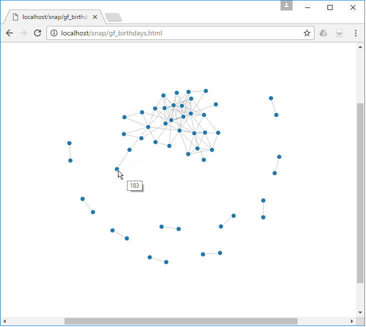
# find all connected vertices with the same birthday identifier
print "same birthdays"
res = g.find("(a)-[]->(b)") \
         .filter("a.birthday = b.birthday")
print "count: %d" % res.count()
display(res.select("a.id", "b.id", "b.birthday"))
Output:
| id | id | birthday |
|---|---|---|
| 56 | 134 | 7 |
| 118 | 134 | 7 |
| 2127 | 2223 | 741 |
| … | … | … |
We can export the table above and display it as a D3 graph. Follow the steps below to export the data from Databricks:
from pyspark.sql.functions import *

# We need to do some heading manipulation so that the two columns named 'id' are changed to 'source' and 'target'
# clean filesystem from previous runs
dbutils.fs.rm("/FileStore/tables/fovepx7h1479410900486/birthdays.csv", True)

# we need Spark to run this job on one node so that only one file is generated.  Thus, we use the coalesce() command
res.select(col("a.id").alias("source"), col("b.id").alias("target")).coalesce(1).write.format("com.databricks.spark.csv").save("/FileStore/tables/fovepx7h1479410900486/birthdays.csv")

# Lists the file generated
dbutils.fs.ls("/FileStore/tables/fovepx7h1479410900486/birthdays.csv")
Once we download the csv file, we can use it to display the data using D3:
Similarly, we can run other graph queries to return different data. Here are to other examples:
# find "friends of friends" who are not connected to us, but graduated the same
# year from the same school
print "same class"
res = g.find("(a)-[]->(b); (b)-[]->(c); !(a)-[]->(c)") \
         .filter("a.education_school_id = c.education_school_id and " \
                 "a.education_year_id = c.education_year_id")
res = res.filter("a.id != c.id").select(col("a.id").alias("source"), "a.education_school_id", "a.education_year_id",
        col("c.id").alias("target"), "c.education_school_id", "c.education_year_id")

# Run PageRank on our graph
pgr = g.pageRank(resetProbability=0.15, tol=0.01).vertices.sort(
    	    'pagerank', ascending=False)
display(pgr.select("id", "pagerank"))
Output:
| id | pagerank |
|---|---|
| 1911 | 17.706611805364975 |
| 3434 | 17.686970750250747 |
| 2655 | 17.117129849434875 |
| … | … |
Clounce hopes that you took some good points from the above. Until the next blog entry, take care and be kind to humanity!