
Mathematica is a computational, mathematics, tool. It is shipped free with Raspberry Pi. In this blog entry, we will look at some basic functions to get you started quick on the subject.
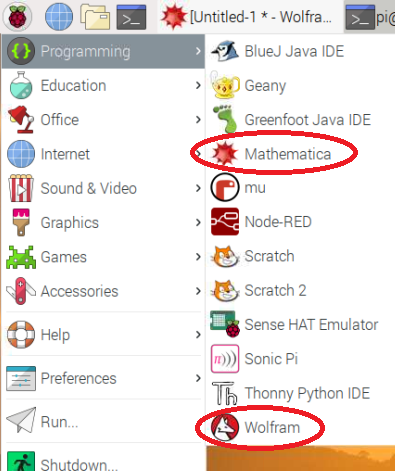
To fire up Mathematica on Raspberry Pi, either click on the Mathematica icon or on the Wolfram icon for command line interface (see image below). Alternatively, you can run Wolfram from the terminal by typing wolfram at the command prompt.
Now that we launched our Mathematica interface, let’s have some fun!
It is a must that you cheer the world from Mathematica, so type Print["Hello World!"] at the wolfram prompt. Here is the result:
 pi@raspberrypi:~ $ wolfram
 Mathematica 12.0.1 Kernel for Linux ARM (32-bit)
 Copyright 1988-2019 Wolfram Research, Inc.
 In[1]:= Print["Hello World!"]
  Hello World!
Next, let’s do some basic arithmetic:
 In[2]:= 2 + 3
  Out[2]= 5

 In[3]:= 33 * 37
  Out[3]= 1221

 In[4]:= 1/(2+2)
          1
  Out[4]= -
          4
Note that for precision purposes Mathematica returned the result of our last expression in fraction format. You can view the numeric equivalent by using the N[] function. By default, Mathematica displays the value up to 6 significant figures. However, this can be overridden by specifying the significant places in the N[] function. The (* ... *) are inline comments. Example:
In[5]:= N[1/(2+2)]
 Out[5]= 0.25

In[6]:= N[1/3]
 Out[6]= 0.333333

In[7]:= N[1/33, 2] (* specify 2 significant places *)
 Out[7]= 0.030

In[8]:= N[Sqrt[2]]
 Out[8]= 1.41421

In[9]:= N[1/Sqrt[2]]
 Out[9]= 0.707107

In[10]:= Sqrt[-25] (* Use of complex numbers *)
 Out[10]= 5 I
Mathematica can help you also in your trigonometry. For example:
In[1]:= Cos[Pi]
 Out[1]= -1

In[2]:= Sin[45 Degree]
            1
 Out[2]= -------
         Sqrt[2]
Note that trig functions expect radian values as parameters. You can use degrees as your input by specifying Degree in your arguments.
You can also ask Mathematica to simplify or solve any mathematical equation. See examples below.
In[16]:= Simplify[Sin[x]^2 + Cos[x]^2]
 Out[16]= 1

In[17]:= TrigReduce[Sin[x]^2 + 2 * Cos[x]^2]
          3 + Cos[2 x]
 Out[17]= ------------
               2

In[28]:= Solve[x^2 + 2x + 2 == 0, x]
 Out[28]= {{x -> -1 - I}, {x -> -1 + I}}

In[29]:= Solve[ 2*a*x + y == 1 && b*x - y == 3, {x, y}]
                    4            6 a - b
 Out[29]= {{x -> -------, y -> -(-------)}}
                 2 a + b         2 a + b
We end this short and quick overview by plotting some nice graphs.
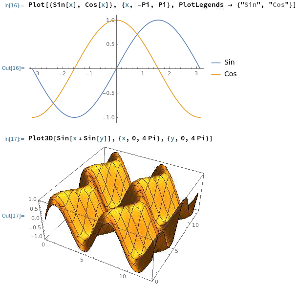
Clounce hopes that this short and light introduction to Mathematica helps you to get started quickly. Mathematica is much more powerful and complex than described above, and it can be used to solve very simple equations like the ones used above or to solve complex differential equations and advanced physics problems. Enjoy and have fun with mathematics!