
In this blog entry we take a look how to highlight a row in a Microsoft Excel table based on a cell value. First we take a look at the steps required and then we take an example to see it in practice. We will use the “Conditional Formatting” feature of Microsoft Excel.
Steps to highlight a row in Microsoft Excel:
- Select the data (table) you want to apply the highlight to.
- Go to the “Conditional Formatting” option and select “New Rule”.
- Select the “Use a formula to determine which cells to format”.
- Put in the formula: =INDIRECT(“<column>”&ROW())=<value>. Where column is the column of which the value is to be compared, and value is the value to compare to.
- Click on the “Format” button to specify how you want the row highlighted.
- Click “Ok”.
Example
Let’s take a look how this is done in practice. For this example we will use a table with Projected and Actual costs for Project X. We want to highlight the row that indicates the cost of the current week. A sample table is show in Figure 1.
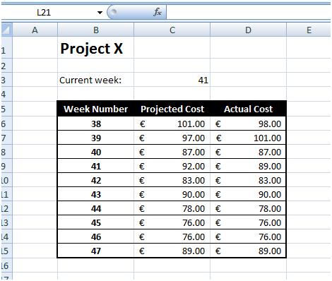
Figure 1: Sample table
Step 1
Select the table you want to format:
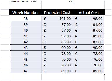
Figure 2: Table selection
Step 2
Go to the “Conditional Formatting” option and select “New Rule”.
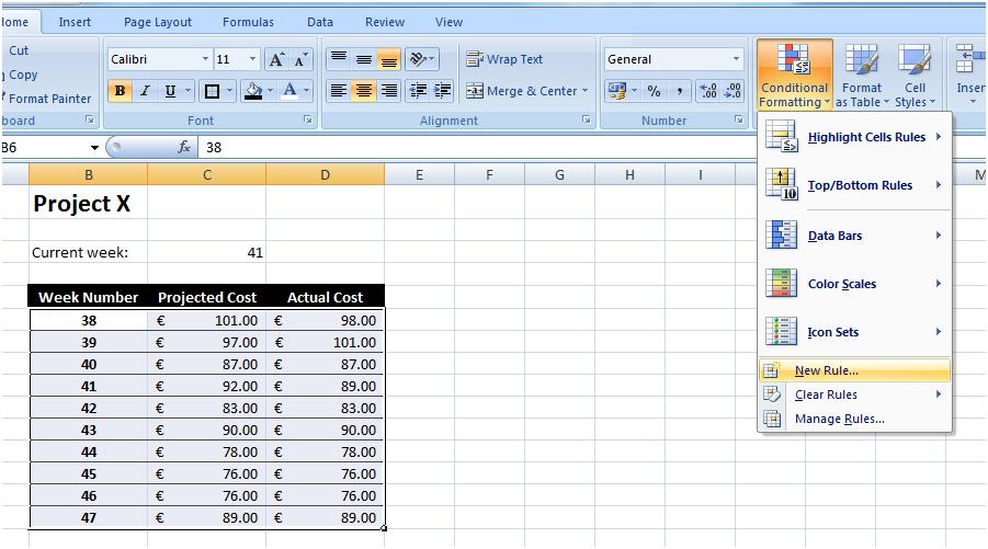
Figure 3: Selecting “New Rule...” from the “Conditional Formatting” option
Step 3
Select the “Use a formula to determine which cells to format”.
Step 4
Put in the formula: =INDIRECT(“B”&ROW())=$C$3. See Figure 4. Note that “B” is the column we want to compare and cell $C$3 contains the value we want to compare to. The value of this cell is automatically updated every week with the week number. To do this we use the formula =WEEKNUM(NOW(),2) as indicated in Figure 5. If for example, you want to highlight all the rows that have a future week number, that is, all those whose week number is greater than the current week number, you will replace the equal comparison (=) to a greater than (>) comparison. Then, the formula will read =INDIRECT(“B”&ROW())>$C$3.
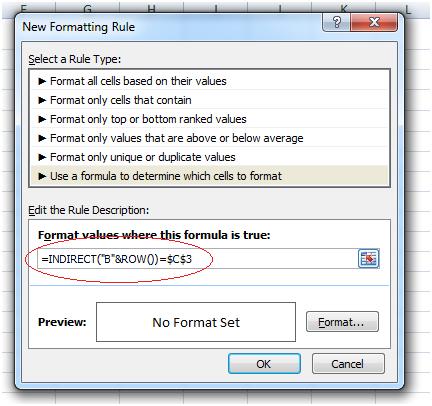
Figure 4: Typing in the formula
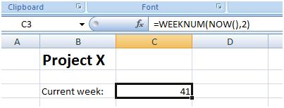
Figure 5: Formula to display the current week’s number
Step 5
The final step is to select the way you want to format your row.

Figure 6: Row formatting
Step 6
When you are satisfied with the formatting, hit the OK button and you are done. Figure 7 shows the final result.
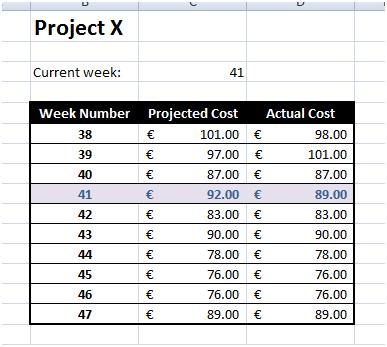
Figure 7: Final result